data_processing module

The data_processing script contains all methods which, as the name suggests, involve data processing. This is important to decouple the hardware classes, GUI elements and other layer of the software architecture from each other. The data_processing module does not only contain independent methods but also separate classes.

Overview:

Independent Methods:

1. Utility Methods:

   • convert_fs_to_mm

   • convert_mm_to_fs

2. Phase Cycling Methods:

   • calculate_interleave_array

   • get_wobbler_states

3. Methods for Time Domain Experiments:

   • find_wavegen_params

   • find_t_zero

   • calculate_counter_values

   • process_ft2dir_data

   • apodization_function

   • process_interferogram

   • calculate_frequency_axis

   • find_opa_range

   • calculate_phase_slope

   • find_zerobin

4. Methods for Data Handling:

   • sort_data

   • shot_to_shot_signal

   • shot_to_shot_viper

5. Visualization Methods for Plotting: * generate_img_data * scale_img * generate_contour_lines * update_contour_lines

Classes:

1. PixelResponseLinearization:

   • _linearize_cubicfraction

   • _linearize_cubic

   • _linearize_one

2. ChopperStateFinder:

   • get_chopper_states

class ChopperStateFinder(path)

Bases: object

Provides functionality to identify which combination of chopper states was present for an input channel that mixes (adds up) the voltage level of a combination of choppers.

The class first loads all necessary information from a json file that specifies the voltage range and name of all choppers. It then creates an array containing all possible combinations of chopper states. This array is then used to calculate bin reference values for the numpy.digitize function.

Note

At the moment the class only provides functionality to digitize the different chopper states. Functionality to identify which choppers had a HIGH signal is fairly easy by using the self.deconvolution_matrix indexed with the return of the np.digitize function. It is not clear if this is needed at the moment thats why it is left out.

Parameters

path (str) – Path to the json file that contains the chopper configuration for the experiment.

chopper_names

Names of the choppers, ordered such that the chopper with the highest voltage value is listed first. This corresponds to the order of the columns of deconvolution matrix.

Type

list

number_of_choppers

Number of choppers specified/characterised in json file. Corresponds to the number of choppers needed for the experiment.

Type

int

deconvolution_matrix

Array containing all possible combinations of chopper states.

• shape: (2^number_of_choppers, number_of_choppers). The 0th column represents the chopper with the highest voltage. This coincides with the chopper_names list

• E.g.: the 1st entry of chopper_names corresponds to the chopper represented by the 1st column of deconvolution matrix.

Type

ndarray

bin_reference_values

Half way points between to adjacent voltage states. This is used by the np.digitize function.

Type

ndarray

get_chopper_states(chopper_adc_data: numpy.ndarray) → numpy.ndarray

Digitizes voltage data of convoluted chopper reference signal into integers that can be used to sort the adc data.

Parameters

chopper_adc_data (ndarray) –

Analog voltage data from chopper input channel of adc.

• shape: 1D

• E.g.:(adc.samples_to_acquire)

Returns

Array that represents each respective voltage state as an integer.

Indexing self.deconvolution_matrix with this array will return the respective state for each chopper for each data point.

• shape: 1D

• E.g.: (adc.samples_to_acquire)

Return type

ndarray

class PixelResponseLinearization(path)

Bases: object

Provides functionality to linearize the MCT pixel response to light intensity.

This class offers functionality to linearize the response of the MCT detector (and its preamplifiers etc.) to changing light intensity.

For object instantiation a JSON file with the fit parameters has to be specified. The top level of the JSON file has two entries, one ‘type’ (str) describing the type of linearization, that is, the fit function, and one dict under the name ‘parameters’, containing either a) the specific linearization parameters for each pixel (dict is large), or one set of parameters to be used for all pixels. During loading, the two cases are handled automatically depending on the size of the ‘parameters’ dict. See below for an example on how an entry of the pixel linearization parameter dict looks like

{
    "0": {
        "name": "Probe (bottom) pixel 0",
        "a": [
            9.7706e-16,
            "float",
            "unitless",
            "fit parameter a from equation Intensity=b*ADC^3+a*ADC+c"
        ],
        "b": [
            1.3441e-05,
            "float",
            "unitless",
            "fit parameter b from equation Intensity=b*ADC^3+a*ADC+c"
        ],
        "c": [
            0.005075,
            "float",
            "unitless",
            "fit parameter c from equation Intensity=b*ADC^3+a*ADC+c"
        ]
    },
    ...
}

The object method linearize is then set up according to the ‘type’ specified in the JSON file by picking one of the preimplemented functions.

Parameters

path (path) – Path to the json file that specifies the fit paramters. The code will automatically detect whether one set of parameters for all pixels or one set of parameters was provided for each pixel.

a,b,c

Fit parameters. The specific meaning depends on the fit function, and there could be more than three. They are there for the use of the fit function only and should not be accessed directly.

• shape: (number_of_mct_pixels) or (1) if only one set of parameters is specified for all pixels.

Type

ndarray

Warning

The fit parameters are generally only valid for the given settings of the pre-amplifiers and the ADC for which the calibration was done. If, for example, the gain is changed a new calibration measurement needs to be done.

References

Datasheets and Manuals/Pixel correction/pixel_linearisation.pdf

apodization_function(data_size: int, window: Optional[str] = None) → numpy.ndarray

Generate an envelope for time domain data to prevent artifacts like Leakage in FFT.

This is essentially a wrapper around the scipy.signal.windows get_window() function. Additionally, the return of a cosine squared window to the existing windows. If no window is specified, an array filled with ones is returned. For some of the windows functions additional parameters need to be provided.

E.g. for a Gaussian envelope the width (standard deviation) needs to be specified. In this case instead of a string, a Tuple needs to passed to window.

Note

If you want to add additional windows not provided by the get window function you can implement the wanted functionality by adding more if clauses.

References

Hamm, Zanni 2011 - Concepts and Methods of 2D Infrared Spectroscopy Section 9.5.7

Werner Herres and Joern Gronholz: Understanding FT·IR Data Processing Part 2

https://en.wikipedia.org/wiki/Window_function

scipy.signal.windows.get_window

Parameters

• data_size (int) – size/ length of the axis on which the fourier transform is performed. I.e.: If we have 64 Pixels and a coresponding data set which has the shape: (64, 1000) we want to perform the Fourier Transform along the last axis. And thus our data_size is 1000.

• window (str or tuple, optional) – Name of the window to use. See scipy.signal.windows.get_window Documentation for choices. For some of the windows functions additional parameters need to be provided. Self implemented choices: cos_square. Defaults to None (effectiveley resulting in an array full of ones).

Returns

envelope/ apodization function with which to multiply time domain data.

• shape: (data:size)

Return type

ndarray

calculate_counter_values(data: numpy.ndarray, r2r_indices: numpy.ndarray, bin_reference_values: numpy.ndarray) → numpy.ndarray

Determines the interferometer position from the (counter) values that the ADC collected from the R-2R-Network.

The counter electronics from Zurich outputs the position via USB (on command) and also on a 16 line parallel port for every laser trigger. The results in a 16 digit binary number that is then converted into 4 digit hexadecimal number. Which is output on a 4 line parallel port. (Interferometer counter box BNC R-2R 1-4, BNC R-2R 5-8 etc.). This data is recorded by the ADC. To obtain the actual counter values we need to decode the analog voltages that the ADC recorded. This is achieved by binning the data from all four channels accordingly using an array containing reference values and the function np.digitize. These reference values have to be measured manually from the R-2R Network by applying 5V to different R2R inputs and recording the corresponding output voltages. These values have to be written in a .csv file (see existing files). The resulting hexadecimal values for each line are then modified to match their poisition in the hexadecimal tetrade using the function np.left_shift. BNC R-2R 1-4 is interpreted to be the channel containing the least significant digit (and so on). Finally, we get the counter position by summation of all four hexadecimal numbers. We now need to divide by 2 because apparently the circuit counts the zero crossings for both photodiodes. (Technically it only makes to count on one photodiode, because the actual resolution is determined by the HeNe Wavelength.) Afterwards we floor the values to obtain integers. Note this is not mentioned in the datasheet and apparently is a empirically determined phenomenon (to understand how to prove that the flooring and division by two is correct see the comments within the code).

References

H-Lab reference values for R2R-Network.csv

TimingScheme.pdf

Counter für Interferometer; Anleitung; Manual; Universitaet Zuerich.pdf

Parameters

• data (ndarray) –

  Complete data set from adc (including pixel data, wobbler, R2R etc.) The indices/ rows containing the information of the R2R are selected automatically.

  • shape: 2D

  • E.g. (number of channels, samples to acquire)

• r2r_indices (ndarray) –

  Indices of the rows in the raw data array from adc that correspond to the input channels connected to the R-2R networks.

  • shape: 1D

  • E.g. (4) the counter is connected to 4 R-2R networks

• bin_reference_values (ndarray) –

  Reference values for each of the R-2R networks.

  • shape: 2D (4, 15) 4 rows for each of the R-2R Networks, 15 values for the 16 levels of the R-2R.

Note

This function was copied from the interferometer_counter module, because it is necessary to be able to call this function without a reference to the actual InterferometerCounter class. This is due to issues regarding pickling within multiprocesses.

Returns

array containing interferometer position in counts.

• shape: (adc.samples_to_acquire)

Return type

ndarray

calculate_frequency_axis(interferogram_size: int, he_ne_wavelength: float = 632.8) → numpy.ndarray

Calculates the frequency axis (pump axis) for a given size of a time domain interferogram.

Parameters

• interferogram (int) – Size of the interferogram data array.

• he_ne_wavelength (float, optional) – Wavelength of the He-Ne-Laser in nanometers that is used to keep track of the position of the moving interferometer arm. Defaults to 632.8 nm.

Returns

Frequency axis (pump axis).

Return type

ndarray

Notes

The resolution/spacing of the frequency domain information and its corresponding axis it given by:

where N is the number of bins that were traversed by the moving arm of the interferometer and is the distance between two adjacent bins.

References

Werner Herres and Joern Gronholz: Understanding FT·IR Data Processing Part 1 (p.2 equation 4)

calculate_interleave_array(interleaves: int, pump_wavelength: float, delay: float) → numpy.ndarray

Generate interleave delay positions.

Interleaves are positions of the delay stage within one wavelength of the pump frequency. We use the interleaves to suppress interference on the MCT detector caused by scattering or similar phenomena. When moving the delay stage a specific delay, we have to additionally move the delay stage in small steps around this delay. These small steps are what we call interleaves and because they are within one cycle of the wavelength this effectively changes the phase of the pump pulse. This change in phase leads to the interference being cancelled out when averaging the interleaves.

Parameters

• interleaves (int) – Number of interleaves to measure.

• pump_wavelength (float) – Wavelength of the pump pulse in nanometers.

• delay (float) – Population delay that is being targeted in femtoseconds.

Returns

absolute interleave positions (delay + respective interleave)

in femtoseconds.

• shape: 1D (interleaves)

Return type

ndarray

calculate_phase_slope(interferogram: numpy.ndarray, frequency_axis: numpy.ndarray, zerobin_guess: int, opa_fwhm_range: numpy.ndarray)

Calculate the phase and its slope for a given zerobin guess of the interferogram.

The data points in the interferogram before the zerobin guess are shifted to the end of the array prior to performing the Fourier Transform. The interferogram is now in the frequency domain and the phase can be calculated. A linear regression of the phase in between the FWHM of the OPA peak is performed to obtain the slope of the phase. To obtain the zerobin the phase should be as close to zero as possible.

Parameters

• interferogram (ndarray) –

  Interferogram data. Contains a voltage for every bin measured by the pyro-detector.

  • shape: 1D

  • E.g.: (interferogram.size)

• frequency_axis (ndarray) –

  Frequency axis (pump axis).

  • shape: 1D

  • E.g.: (interferogram.size/2)

• zerobin_guess (int) – Guess for the zerobin as index of the interferogram.

• opa_fwhm_range (ndarray) –

  Indices for all data points in between the FWHM of the pump OPA pulse.

  • shape: 1D

Returns

Slope of the phase (from linear regression).

Return type

float

convert_fs_to_mm(femtoseconds: float)

Converts femtoseconds to millimeters.

Parameters

femtoseconds (float) – Value in femtoseconds.

Returns

Value in millimeters.

Return type

float

convert_mm_to_fs(mm: float)

Converts femtoseconds to millimeters.

Parameters

mm (float) – Value in millimeters.

Returns

Value in femtoseconds.

Return type

float

find_opa_range(spectrum: numpy.ndarray)

Find characteristics of OPA pulse: center position (index), indices of peak, and indices of full width half maximum (fwhm).

The algorithm first truncates the spectrum s.t. it starts at the first index. The 0th index is ignored because the Fourier Transform yields the sum of all values of the interferogram. This can lead to an “unnatural” peak at the 0th position that we are not interested in. The scipy.signal.find_peaks function is used to find all peaks that are higher than 80% of the maximum of the spectrum. Then the scipy.signal.peak_widths function is used to find the width and indices of our peak at 50% height (fwhm) and at 5% height (which we consider to be full width). Then arrays containing all indices within the range of fwhm and full width are generated.

Note

When zero padding the time domain data alot, we sometimes observed that the find_peaks function finds several peaks instead of just one. These peaks are in close proximity to each other and probably are some kind of artifact. In this case, we choose the peak that returns the greater peak width.

Parameters

spectrum (ndarray) –

OPA pump spectrum (generally obtained from Fourier Transform).

• shape: (interferogram.size) size of the zeropadded interferogram

Returns

Contains information about OPA pulse.

center position (index), indices of peak, and indices of full width half maximum (fwhm).

int: index of the of the OPA pulse maximum

ndarray: indices locating the full width of the OPA pulse in spectrum.

• shape: 1D, depends on spectral width of the OPA pulse.

ndarray: indices locating the fwhm of the OPA pulse in spectrum.

• shape: 1D, depends on spectral width of the OPA pulse.

Return type

tuple

find_t_zero(signal, delays)

find_wavegen_params(frequency, no_of_solutions=1, ylimit=4095, force=2, xmin=1000)

Finds optimum wavegen parameters for a desired frequency.

The function returns a list of tuples of integers (x,y) such that the given frequency is optimally approximated by:

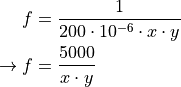x must be between 2 and 4096 (inclusive) and should be as large as possible.

y must be greater than 0. (should be limited at least to x_max)

Parameters

• frequency (float) – value in Hertz

• no_of_solutions (int) – number of solutions (default 1)

• ylimit (int) – maximum y value (default 4095)

• force (int) – force a divisor that x _must_ have

• xmin (int) – lower limit of possible x

Returns

list of pairs of integers

Return type

[(x,y),..]

find_zerobin(interferogram: numpy.ndarray, frequency_axis: numpy.ndarray, zerobin_guess: int, opa_fwhm_range: numpy.ndarray, slope=None)

Determines the zerobin.

Calculates the slope of the phase and searches the zerobin by comparing the slopes. The zerobin guess is incremented by +1 if the slope is negative and by -1 if it is positive (see References). The algorithm checks whether the slope had a sign change to determine when the zerobin was found. Of the two bins where the sign change occured, the one which has a phase slope that is closer to 0 is chosen as zerobin.

Parameters

• interferogram (ndarray) –

  Interferogram data. Contains a voltage for every bin measured by the pyro-detector.

  • shape: 1D

  • E.g. (interferogram.size)

• frequency_axis (ndarray) –

  Frequency axis (pump axis).

  • shape: 1D

  • E.g. (interferogram.size/2)

• zerobin_guess (int) – Guess for the zerobin. Index of the interferogram.

• opa_fwhm_range (ndarray) –

  Indices for all data points in between the FWHM of the pump OPA pulse.

  • shape: 1D

References

Jan Helbing and Peter Hamm: Compact implementation of Fourier transform two-dimensional IR spectroscopy without phase ambiguity

generate_contour_lines(data: numpy.ndarray, img: pyqtgraph.graphicsItems.ImageItem.ImageItem, contour_levels: int = 10)

Generates contour lines for given data.

Sets positive height contour lines to black solid line.

Sets negative height contour lines to black dashed line.

Parameters

• data (ndarray) –

  Data from which to generate contour lines.

  • shape: 2D

• img (pg.ImageItem) – ImageItem to which contour lines will be “attached”/overlayed.

• contour_levels (int, optional) – Number of contour levels to generate. Defaults to 10.

Returns

List holding references to contourline objects

(IsocurveItem). Pass this to the update_contour_lines function to update them.

Return type

list

generate_img_data(x_axis: numpy.ndarray, y_axis: numpy.ndarray, data: numpy.ndarray)

Generates data for heatmap/imshow plot in pyqtgraph.

The returned data set is linearly interpolated to have equal spacing between “real” data points. Because pyqtgraph is not able to plot on unevenly spaced axes. (In matplotlib there exists a function called pcolormesh, just FYI. May later come also to pyqtgraph, see references.)

Parameters

• x_axis (ndarray) – x-axis points (columns) of the data set

• y_axis (ndarray) – y-axis points (rows) of the data set

• data (ndarray) –

  data set that will be transformed into data with respectively equally spaced x- and y-axis data points using linear interpolation.

  • shape: 2D

  • E.g.: (pixels, delays)

References

https://github.com/pyqtgraph/pyqtgraph/issues/1262

https://github.com/pyqtgraph/pyqtgraph/pull/1273

Returns

interpolated data set with x- and y-axis

that are equally spaced respectively.

• shape: 2D

• E.g.: (> pixels, > delays)

Return type

ndarray

get_wobbler_states(wobbler_adc_data: numpy.ndarray, laser_freq: float, wobbler_freq: float = 250) → numpy.ndarray

Assigns each state/position of the wobbler a number 0,1,2,3…

The number 0 indicated that the Wobbler-Voltage was at the maximum value. This method assumes that values oscillate perfectly, with no skipping.

Note

This will only work if the wobbler frequency is 1/4 of the laser repetition rate.

Parameters

• wobbler_adc_data (ndarray) –

  Array containing ADC values of the Wobbler. It technically does not matter if these values come directly from the reference coil, or run through the an additional arduino.

  • shape: (adc.samples_to_acquire), other 1D shapes should work fine too.

• laser_freq (float) – laser repition rate in Hz

• wobbler_freq (float, optional) – Resonance frequency of the wobbler in Hz. Defaults to 250 Hz.

Returns

Array containing values 0,1,2,3..

Where 0 corresponds to the maximum Wobbler-Voltage.

• shape: (wobbler_adc_data.size)

Return type

ndarray

process_ft2dir_data(data: numpy.ndarray, interferogram: numpy.ndarray, window_function: Optional[str] = None, zero_pad_factor: int = 2)

Computes the phase corrected 2D-FTIR spectrum from the time domain data of the MCT (or more spefically the probe (pulse) absorption spectrum in the pump time domain) and applies a window function if specified.

Step by Step Algorithm:

1. The interferogram data, collected from the Zurich counter electronics, is used to find the zerobin (the position of the interferometer from which we are interested in the data, which also corresponds to the position where the pump pulses perfectly, temporally overlap). Furthermore the interferogram and the fourier transformed interferogram (pump spectrum) are obtained together with the pump frequency axis and the necessary information to find the pump OPA pulse within the spectrum

2. The time domain data (absorption spectrum) is shortened such that it starts at the zerobin position

3. The time domain data (absorption spectrum) is offset corrected

4. The time domain data (absorption spectrum) is zeropadded for better interpolation. For better understanding of zeropadding see references

5. A window function apodization function is calculated and applied to the time domain data.

6. The time domain data is fourier transformed into the frequency domain

7. The phasing factor is calculated from the pump spectrum (which was obtained through the fourier transformed interferogram)

8. The frequency domain data is phase corrected

See also

• process_interferogram

• find_zerobin

• find_opa_range

• apodization_function

• calculate_frequency_axis

References

Werner Herres and Joern Gronholz: Understanding FT·IR Data Processing Part 2

Parameters

• data (ndarray) –

  Array which contains time domain data of probe pulse absorption spectrum. This can be calculated by applying lambert beers law () on the linearized MCT data.

  • shape: (number_of_pixel, interferometer positions)

• interferogram (ndarray) –

  Array containing the interferogram which is used to obtain the pump frequency range and the zerobin (the position of the interferometer from which we are interested in the MCT data).

  • shape: (interferometer positions)

• window_function (str, optional) – Apodization function which is applied to the time domain data. See scipy.signal.windows.get_window Documentation for choices. For some of the windows functions additional parameters need to be provided. Self implemented choices: cos_square. Defaults to None.

• zero_pad_factor (int, optional) – Factor with which we want to zeropad the time domain data. For the algorithm to work properly, a factor of at least 2 is necessary. Defaults to 2.

Returns

Contains frequency domain data and interferogram information

(ndarray, tuple)

ndarray: spectrum_2d contains the frequency domain data from the

mct pixels.

• shape: (number_of_pixels, zero padded time domain data size)

tuple: interferogram_information contains the zerobin, the

interferogram and the fourier transformed interferogram as well as the information which is needed to plot the correct part of the data (in range of the pump OPA pulse). It also contains the pump frequency axis necessary for plotting.

Return type

tuple

process_interferogram(interferogram: numpy.ndarray, zero_pad_factor: int = 2)

Obtain the zerobin, the pulse width of the opa and the frequency axis from an interferogram.

Step by Step Algorithm:

1. The interferogram is offset corrected

2. Take the maximum of the interferogram as the initial guess

3. Zeropad interferogram to have an efficient length for Fourier Transform

4. Obtain the amplitude of the Fourier Transform of the interferogram

5. Determine full width half maximum (fwhm) indices of the OPA pump-spectrum as reference values where the phase is linear. This is important because the phase is only linear around the maximum and strongly fluctuates other wise

6. Calculate the phase for different points within fwhm and obtain its derivative/ slope by linear regression

7. The zerobin is the position where the slope of the phase is as close to zero as possible

8. Zeropad interferogram to match zero_pad_factor requirement

9. Compute Fourier Transform of zeropadded interferogram

10. Get the OPA spectrum info: peak (maximum) index, indices of the pulse in the spectrum, indicies of of the fwhm

Parameters

• interferogram (ndarray) –

  Interferogram data. Contains a voltage value for every bin measured by the pyro-detector.

  • shape: 1D

  • E.g. (interferometer positions)

• zero_pad_factor (int, optional) – Factor with which we want to zeropad the time domain data. For the algorithm to work properly, a factor of at least 2 is necessary. Defaults to 2.

Returns

Contains information about the Zerobin and other OPA peak related information

(int, ndarray, ndarray, ndarray, tuple)

int: Zerobin

an index representing the position of the interferometer, where the two pump pulses overlap (temporally).

ndarray: Zero padded, offset corrected, rolled interferogram

The zerobin is the 0th entry of the array and all values in front of the zerobin are shifted to the end of the array.

• shape: 1D

• E.g.: (next_fast_len(interferogram.size*zero_pad_factor))

ndarray: OPA pump-spectrum

obtained from the Fourier Transform of zeropadded interferogram.

• shape: 1D

• E.g.: (zeropadded interferogram size/2)

ndarray: Frequency axis (pump axis)

• shape: 1D

• E.g.: (zeropadded interferogram size/2)

tuple: OPA pulse information

• E.g. Indices/locations of the pump OPA pulse in the spectrum that was obtained from the amplitude (absolute) of the FFT. This can be used to later get the phase at the location of the zerobin and to plot the relevant part of the spectrum (OPA pump-pulse).

Return type

tuple

References

Jan Helbing and Peter Hamm: Compact implementation of Fourier transform two-dimensional IR spectroscopy without phase ambiguity

For better understanding of Fourier Transformation see also:

Werner Herres and Joern Gronholz: Understanding FT·IR Data Processing Part 1 - 3

scale_img(x_axis: numpy.ndarray, y_axis: numpy.ndarray, data: numpy.ndarray, img: pyqtgraph.graphicsItems.ImageItem.ImageItem)

Makes it such that the axes of the image are correctly displayed.

This is achieved by translating / moving the image to the point of the 0 th entries of the x- and y-axis and then scaling it accordingly.

Parameters

• x_axis (ndarray) – x-axis points (columns) of the data set (it does not matter whether this is the interpolated or non-interpolated axis)

• y_axis (ndarray) – y-axis points (rows) of the data set (it does not matter whether this is the interpolated or non-interpolated axis)

• data (ndarray) –

  interpolated data set that was used to generate the ImageItem

  • shape: 2D

• img (pg.ImageItem) – ImageItem that is supposed to be adjusted.

shot_to_shot_signal(transmission: numpy.ndarray, chopper_state: Optional[int] = None)

Calculates the difference absorption spectra for the adjacent samples (shots) in the data and extracts statistical data.

Parameters

• transmission (ndarray) –

  transmisson or relative intensity (probe/ref array) for each pixel from which difference signal should be calculated.

  • shape: 2D

  • E.g. (number of pixels per row, samples to acquire)

• chopper_state (int, optional) –

  1 if the 0th sample (column) in the array corresponds to data from a pumped state.

  0 if the 0th sample (column) in the array corresponds to data from an unpumped state. For data where chopper was not running but a “pseudo signal” should be calculated this argument does not need to be specified. Defaults to None.

Returns

Tuple with data from difference absorption spectra

Containing Averaged shot-to-shot signal, amplitude, standard deviation and average standard deviation of signal

ndarray: Averaged shot-to-shot signal

• shape: 1D (number of pixels per row)

float: Amplitude

Amplitude of the the averaged shot-to-shot signal calculated by subtracting the minimum from the maximum.

ndarray: Standard deviation of shot-to-shot signal

• shape: 1D (number of pixels per row)

float: Average standard deviation of shot-to-shot signal

standard deviation of shot-to-shot signal averaged over all pixels. This is what was referred to as mean noise.

Return type

tuple

shot_to_shot_viper(transmission: numpy.ndarray, vis_chopper_state: int, ir_chopper_state: numpy.ndarray)

Calculates the VIPER difference absorption spectra for 4 adjacent samples (shots) in the data and extracts statistical data.

Parameters

• transmission (ndarray) –

  transmission or relative intensity (probe/ref array) for each pixel from which difference signal should be calculated.

  • shape: 2D

  • E.g. (number of pixels per row, samples to acquire)

• vis_chopper_state (int) –

  1 if the 0th sample (column) in the array corresponds to data from a UV/VIS pumped state.

  0 if the 0th sample (column) in the array corresponds to data from an UV/VIS unpumped state. This assumes that the UV/VIS Chopper runs at half of the laser repitition rate.

• ir_chopper_state (ndarray) –

  • [1, 1] if the 0th and 1st sample (column) in the array corresponds to data from two IR pumped states.

  • [0, 1] if the 0th sample (column) corresponds to an IR unpumped state while the 1st sample (column) corresponds to an IR pumped state.

  • [1, 0] if the 0th sample (column) corresponds to an IR pumped state while the 1st sample (column) corresponds to an IR unpumped state.

  • [0, 0] if the 0th and 1st sample (column) in the array corresponds to data from two IR unpumped states.

Returns

Data from VIPER difference absorption spectrum.

Containing Averaged shot-to-shot VIPER signal, amplitude, standard deviation and average standard deviation of VIPER signal

averaged shot-to-shot VIPER signal (ndarray):

• shape: 1D (number of pixels per row)

amplitude (float):

Amplitude of the the averaged shot-to-shot VIPER signal calculated by subtracting the minimum from the maximum.

standard deviation of shot-to-shot VIPER signal (ndarray):

• shape: 1D (number of pixels per row)

average standard deviation of shot-to-shot VIPER signal (float):

standard deviation of shot-to-shot signal averaged over all pixels. This is what was reffered to as mean noise.

Return type

tuple

sort_data(data: numpy.ndarray, states: numpy.ndarray, number_of_possible_states: numpy.ndarray) → tuple

For each state, average the associated spectral data and return a (multidimensional) array holding those averaged data. Additionally, calculate base statistical information for each state and for each pixel. Also returns weights, which are the inverse of the variance, to use when averaging data from separate acquisitions (see references).

This function takes a 2D array, containing an unsorted series of spectral data (spectral referring to the fact that the data is collected from the spectrometer + MCT).

Each spectrum is labelled with the system’s state variables (e.g. wobbler state, chopper state, polarizer state) via the associated states array. For each shot, the states array records the state of one or more state variables.

The function then sorts and groups the data with identical states and averages them - these are repeat measurements. The individual component states (wobbler, chopper, etc.) serve as indices into this multidimensional array of results. _Crucially, this relies on the states being representable as integers that can serve as array indices.

What is achieved here: we want to average the datapoints / lasershots that belong to the same state of the experiment. The ADC collects the data that we want to sort and average, and labels them also with the information in which state the system was at each recorded shot. In the simplest case the states array is 1D, representing just one discriminating factor, i.e. wobbler position. Our wobbler can be in four different positions, thus we would have a 1D state 1D array, containing the wobbler state for each shot (in this case, a number out of 0, 1, 2 or 3). We now can average all laser shots with wobbler state 0 separately from wobbler state 1 etc.

Now imagine we have a wobbler and an interferometer in our setup. So we effectively have a 2D state array, with two numbers per laser shot. One row contains the position of the interferometer and the other row contains the wobbler state for each laser shot. Now we only want to average data at the same interferometer position and the same wobbler state. So we need to find the indices of all columns in the state array that are identical and then average the data at those indices. Each additional state variable would add another row to this 2D state array.

This function represents a generalized method to achieve this grouping and averaging. By passing a data array and a state array that have both the same number of columns (i. e. shots), we can group corresponding data columns together.

Parameters

• data (ndarray) –

  For frequency-domain data use normalized intensity (transmission). This can be calculated from the linearized ADC data by dividing the probe pixel by the reference pixels. For pump time-domain and probe frequency-domain data (non-normalized) intensity or ADC counts/voltage were used in LabView.

  • shape: 2D

  • E.g.: (number_of_pixels_per_row, samples_to_acquire) or (number_of_pixels, samples_to_acquire) respectively.

  Note:

  Although the algorithm is able to sort the raw, non-normalized data, one should always input transmission values for pure frequency domain data. The reason for this is explained in:

  Brazard, J., Bizimana, L. A., & Turner, D. B. (2015). Accurate convergence of transient-absorption spectra using pulsed lasers. Review of Scientific Instruments, 86(5), 053106. Section 2 Part D.

  Note:

  When comparing the sorting of non-normalized intensities to sorting normalized intensities/transmission for time-domain pump and frequency-domain probe experiments (namely FT-2D-IR) for the same raw data set there was no significant difference. The difference between the two was at least two orders of magnitude smaller than the resulting frequency-domain difference absorption spectrum. There seems to be no reason against sorting shot-to-shot normalized intensities (transmission). We believe this should also generally lead to better data quality.

  Caveat: The raw data set this was tested on only contained negative delays. We recommend investigating this in more depth.

• states (ndarray) –

  2D array containing different parts of the state information for each laser shot in terms of integers:

  1. first row: interferometer positions (0-65535),

  2. second_row: chopper states (0-7),

  3. third_row: wobbler states (0-3).

  • shape: 1D or 2D

  • E.g.: (number_of_state_monitors, samples_to_acquire)

  Note:

  The state information needs to start at 0 and must not exceed the corresponding value specified in number_of_possible_states. I.e.: To achieve this for the interferometer position one can subtract the minimum so that the lowest count is 0 and one can obtain the values for number_of_possible_states by taking the maximum and adding 1.

• number_of_possible_states (ndarray) –

  For each row in states the number of possible states that this state monitor reaches.

  • shape: 1D (number_of_state_monitors)

  • E.g.: np.array([65536, 8, 4]) (taking the example from states docstring).

Returns

Contains information for each state.

Contains sorted and averaged data for each state, weights, counts and statistical data

ndarray: sorted and averaged data.

• shape: Multidimensional e.g. (number_of_pixels_per_row, number of interferometer positions, number of chopper states, number of wobbler states)

ndarray: weights (inverse variance) for each state to use when averaging two

different scans/acquisitions.

• shape: Multidimensional, same size as sorted_data

• I.e. (number_of_pixels_per_row, number of interferometer positions, number of chopper states, number of wobbler states)

ndarray: counter: how often a given state was found in the unsorted data. This can be

used for trouble shooting to see if all states were ‘hit’.

• shape: Multidimensional - one dimension less than the averaged data.

• E.g.: (number of interferometer positions, number of chopper states, number of wobbler states)

tuple of pd.DataFrame: base statistical data:

(variance, mean_state_std, mean_state_std_std)

1. variance: the variance for all states and all pixels/transmission values

2. mean_state_std: mean standard deviation of all states for all pixels, this indicates how much the laser intensity fluctuated during the acquisition for a given pixel. Use this to visualize the fluctuations of the laser.

3. std_state_std: standard deviation of standard deviation of all states for all pixels, this indicates how much the fluctuation of the laser intensity varied with the states. Use this as errorbars when plotting the fluctuations of the laser.

Return type

tuple

Note

The computational time needed for this algorithm to run depends largely on the size of the data set (samples_to_acquire) and also on the total number of possible states. It is recommended to reduce this number as far as possible. This is, for instance, very relevant for the interferometer positions since we only move the interferometer in a small range. If the counter of the interferometer has been reset appropriately the maximum count we are going to record will be approximately 4000. So the function will run a lot faster if we provide number_of_possible_states with 4001 (yes, 4000+1) instead of 65536. Also make sure you have enough RAM in the computer. We encountered a sudden (unproportional) increase in runtime when increasing the size of the data. We could trace this back to the RAM that python needs.

References

Brazard, J., Bizimana, L. A., & Turner, D. B. (2015). Accurate convergence of transient-absorption spectra using pulsed lasers. Review of Scientific Instruments, 86(5), 053106.

https://en.wikipedia.org/wiki/Weighted_arithmetic_mean#Variance_weights

update_contour_lines(data: numpy.ndarray, contour_lines: list)

Update contour lines given the new data set.

Parameters

• data (ndarray) –

  Data from which to generate contour lines.

  • shape: 2D

• contour_lines (list) – List of IsocurveItem references.